Petri net
A Petri net (also known as a place/transition net or P/T net) is one of several mathematical modeling languages for the description of distributed systems. A Petri net is a directed bipartite graph, in which the nodes represent transitions (i.e. events that may occur, signified by bars) and places (i.e. conditions, signified by circles). The directed arcs describe which places are pre- and/or postconditions for which transitions (signified by arrows). Some sources[1] state that Petri nets were invented in August 1939 by Carl Adam Petri – at the age of 13 – for the purpose of describing chemical processes.
Like industry standards such as UML activity diagrams, BPMN and EPCs, Petri nets offer a graphical notation for stepwise processes that include choice, iteration, and concurrent execution. Unlike these standards, Petri nets have an exact mathematical definition of their execution semantics, with a well-developed mathematical theory for process analysis.
Petri net basics
A Petri net consists of places, transitions, and arcs. Arcs run from a place to a transition or vice versa, never between places or between transitions. The places from which an arc runs to a transition are called the input places of the transition; the places to which arcs run from a transition are called the output places of the transition.
Graphically, places in a Petri net may contain a discrete number of marks called tokens. Any distribution of tokens over the places will represent a configuration of the net called a marking. In an abstract sense relating to a Petri net diagram, a transition of a Petri net may fire whenever there are sufficient tokens at the start of all input arcs; when it fires, it consumes these tokens, and places tokens at the end of all output arcs. A firing is atomic, i.e., a single non-interruptible step.
Execution of Petri nets is nondeterministic: when multiple transitions are enabled at the same time, any one of them may fire. If a transition is enabled, it may fire, but it doesn't have to.
Since firing is nondeterministic, and multiple tokens may be present anywhere in the net (even in the same place), Petri nets are well suited for modeling the concurrent behavior of distributed systems.
Formal definition and basic terminology
Petri nets are state-transition systems that extend a class of nets called elementary nets.[2]
Definition 1. A net is a triple N = (P, T, F ) where:
- P is a set of states, called places.
- T is a set of transitions.
- F where F ⊂ (P × T ) ∪ (T × P ) is a set of flow relations called "arcs" between places and transitions (and between transitions and places). A net is a bipartite graph, where P is one partition and T is the other. Moreover, for every t in T there exist p and q in P so that (p, t) and (t, q) are in F and for every p and q in P, if (p, t) and (t, q) are in F then p ≠ q.
The set P ∪ T are the net elements. The set of places define the local states of a net, however, the global state of a net can be defined by place subsets.
Definition 2. Given a net N = (P, T, F ), a configuration is a set C so that C ⊆ P.
Definition 3. An elementary net is a net of the form EN = (N, C ) where:
- N = (P, T, F ) is a net.
- C is such that C ⊆ P is a configuration.
Definition 4. A Petri net is a net of the form PN = (N, M, W ), which extends the elementary net so that:
- N = (P, T, F ) is a net.
- M so that M : P → Z is a place multiset, where Z is a countable set. M extends the concept of configuration and is commonly described with reference to Petri net diagrams as a marking.
- W so that W : F → Z is an arc multiset, so that the count for each arc is a measure arc multiplicity.
If a Petri net is equivalent to an elementary net, then Z can be the countable set {0,1} and those elements in P that map to 1 under M form a configuration. Similarly, if a Petri net is not an elementary net, then the multiset M can be interpreted as representing a non-singleton set of configurations. In this respect, M extends the concept of configuration for elementary nets to Petri nets.
In the diagram of a Petri net (see top figure left), places are conventionally depicted with circles, transitions with long narrow rectangles and arcs as one-way arrows that show connections of places to transitions or transitions to places. If the diagram were of an elementary net, then those places in a configuration would be conventionally depicted as circles, where each circle encompasses a single dot called a token. In the given diagram of a Petri net (see left), the place circles may encompass more than one token to show the number of times a place appears in a configuration. The configuration of tokens distributed over an entire Petri net diagram is called a marking.
In the top figure (see left), the place p1 is an input place of transition t; whereas, the place p2 is an output place to the same transition. Let PN0 (Fig. top) be a Petri net with a marking configured M0 and PN1 (Fig. bottom) be a Petri net with a marking configured M1. The configuration of PN0 enable transition t through the property that all input places have sufficient number of tokens (shown in the figures as dots) "equal to or greater" than the multiplicities on their respective arcs to t. Once and only once a transition is enabled will the transition fire. In this example, the firing of transition t generates a map that has the marking configured M1 in the image of M0 and results in Petri net PN1, seen in the bottom figure. In the diagram, the firing rule for a transition can be characterised by subtracting a number of tokens from its input places equal to the multiplicity of the respective input arcs and accumulating a new number of tokens at the output places equal to the multiplicity of the respective output arcs.
Remark 1. The precise meaning of "equal to or greater" will depend on the precise algebraic properties of addition being applied on Z in the firing rule, where subtle variations on the algebraic properties can lead to other classes of Petri nets; for example, Algebraic Petri nets (see[3]).
The following formal definition is loosely based on (Peterson 1981). Many alternative definitions exist.
Syntax
A Petri net graph (called Petri net by some, but see below) is a 3-tuple  , where
- S is a finite set of places
- T is a finite set of transitions
- S and T are disjoint, i.e. no object can be both a place and a transition
 is a multiset of arcs, i.e. it assigns to each arc a non-negative integer arc multiplicity; note that no arc may connect two places or two transitions.
The flow relation is the set of arcs:  . In many textbooks, arcs can only have multiplicity 1. These texts often define Petri nets using F instead of W. When using this convention, a Petri net graph is a bipartite multigraph
  with node partitions S and T.
The preset of a transition t is the set of its input places: 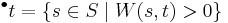 ; its postset is the set of its output places:
 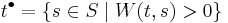 . Definitions of pre- and postsets of places are analogous.
A marking of a Petri net (graph) is a multiset of its places, i.e., a mapping  . We say the marking assigns to each place a number of tokens.
A Petri net (called marked Petri net by some, see above) is a 4-tuple  , where
 is a Petri net graph;
 is the initial marking, a marking of the Petri net graph.
Execution semantics
The behavior of a Petri net is defined as a relation on its markings, as follows.
Note that markings can be added like any multiset: 
The execution of a Petri net graph  can be defined as the transition relation
  on its markings, as follows:
- for any t in T:

In words:
- firing a transition t in a marking M consumes
 tokens from each of its input places s, and produces
  tokens in each of its output places s
 - a transition is enabled (it may fire) in M if there are enough tokens in its input places for the consumptions to be possible, i.e. iff
 .
.
We are generally interested in what may happen when transitions may continually fire in arbitrary order.
We say that a marking  is reachable from a marking M in one step if
  ; we say that it is reachable from M if
  , where
  is the reflexive transitive closure of
  ; that is, if it is reachable in 0 or more steps.
For a (marked) Petri net  , we are interested in the firings that can be performed starting with the initial marking . Its set of reachable markings is the set
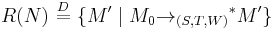
The reachability graph of N is the transition relation restricted to its reachable markings  . It is the state space of the net.
A firing sequence for a Petri net with graph G and initial marking is a sequence of transitions 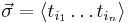 such that
  . The set of firing sequences is denoted as
  .
.
Variations on the definition
As already remarked, a common variation is to disallow arc multiplicities and replace the bag of arcs W with a simple set, called the flow relation, 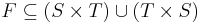 . This doesn't limit expressive power as both can represent each other.
Another common variation, e.g. in, e.g. Desel and Juhás (2001),[4] is to allow capacities to be defined on places. This is discussed under extensions below.
Formulation in terms of vectors and matrices
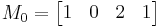
The markings of a Petri net can be regarded as vectors of nonnegative integers of length  .
.
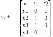
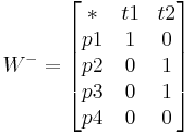
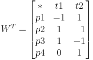
Its transition relation can be described as a pair of by  matrices:
 , defined by
 ![\forall s,t: W^-[s,t] = W(s,t)](/2012-wikipedia_en_all_nopic_01_2012/I/8ba8d38671262e895920e4cc2391cd18.png)
 , defined by
 ![\forall s,t: W^%2B[s,t] = W(t,s).](/2012-wikipedia_en_all_nopic_01_2012/I/8f87c9b3aab9624bb8af0a6c21edcab1.png)
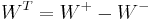
Then their difference
can be used to describe the reachable markings in terms of matrix multiplication, as follows. For any sequence of transitions w, write  for the vector that maps every transition to its number of occurrences in w. Then, we have
 is a firing sequence of
  .
.
Note that it must be required that w is a firing sequence; allowing arbitrary sequences of transitions will generally produce a larger set.
Mathematical properties of Petri nets
One thing that makes Petri nets interesting is that they provide a balance between modeling power and analyzability: many things one would like to know about concurrent systems can be automatically determined for Petri nets, although some of those things are very expensive to determine in the general case. Several subclasses of Petri nets have been studied that can still model interesting classes of concurrent systems, while these problems become easier.
An overview of such decision problems, with decidability and complexity results for Petri nets and some subclasses, can be found in Esparza and Nielsen (1995).[5]
Reachability
The reachability problem for Petri nets is to decide, given a Petri net N and a marking M, whether  .
.
Clearly, this is a matter of walking the reachability graph defined above, until either we reach the requested marking or we know it can no longer be found. This is harder than it may seem at first: the reachability graph is generally infinite, and it is not easy to determine when it is safe to stop.
In fact, this problem was shown to be EXPSPACE-hard[6] years before it was shown to be decidable at all (Mayr, 1981). Papers continue to be published on how to do it efficiently.[7]
While reachability seems to a be a good tool to find erroneous states, for practical problems the constructed graph usually has far too many states to calculate. To alleviate this problem, linear temporal logic is usually used in conjunction with the tableau method to prove that such states cannot be reached. LTL uses the semi-decision technique to find if indeed a state can be reached, by finding a set of necessary conditions for the state to be reached then proving that those conditions cannot be satisfied.
Liveness
Petri nets can be described as having different degrees of liveness  . A Petri net
  is called
  -live iff all of its transitions are -live, where a transition is
- dead, iff it can never fire, i.e. it is not in any firing sequence in

 -live (potentially fireable), iff it may fire, i.e. it is in some firing sequence in
  -live iff it can fire arbitrarily often, i.e. if for every positive integer k, it occurs at least k times in some firing sequence in
  -live iff it can fire infinitely often, i.e. if for every positive integer k, it occurs at least k times in V, for some prefix-closed set of firing sequences
 -live (live) iff it may always fire, i.e., it is -live in every reachable marking in
  )
)
Note that these are increasingly stringent requirements:  -liveness implies
  -liveness, for
  .
.
These definitions are in accordance with Murata's overview,[8] which additionally uses  -live as a term for dead.
Boundedness
A place in Petri net is called k-bounded if it does not contain more than k tokens in all reachable markings, including the initial marking; it is safe if it is 1-bounded; it is bounded if it is k-bounded for some k.
A (marked) Petri net is called k-bounded, safe, or bounded when all of its places are. A Petri net (graph) is called (structurally) bounded if it is bounded for every possible initial marking.
Note that a Petri net is bounded if and only if its reachability graph is finite.
Boundedness is decidable by looking at covering, by constructing the Karp–Miller Tree.
It can be useful to explicitly impose a bound on places in a given net. This can be used to model limited system resources.
Some definitions of Petri nets explicitly allow this as a syntactic feature.[9] Formally, Petri nets with place capacities can be defined as tuples 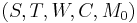 , where
 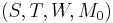 is a Petri net,
  an assignment of capacities to (some or all) places, and the transition relation is the usual one restricted to the markings in which each place with a capacity has at most that many tokens.
For example, if in the net N, both places are assigned capacity 2, we obtain a Petri net with place capacities, say N2; its reachability graph is displayed on the right.
Alternatively, places can be made bounded by extending the net. To be exact, a place can be made k-bounded by adding a "counter-place" with flow opposite to that of the place, and adding tokens to make the total in both places k.
Discrete, continuous, and hybrid Petri nets
As well as discrete events, there are Petri nets for continuous and hybrid discrete-continuous processes and useful in discrete, continuous and hybrid control theory.[10] and related to discrete, continuous and hybrid automata.
Extensions
There are many extensions to Petri nets. Some of them are completely backwards-compatible (e.g. coloured Petri nets) with the original Petri net, some add properties that cannot be modelled in the original Petri net (e.g. timed Petri nets). If they can be modelled in the original Petri net, they are not real extensions, instead, they are convenient ways of showing the same thing, and can be transformed with mathematical formulas back to the original Petri net, without losing any meaning. Extensions that cannot be transformed are sometimes very powerful, but usually lack the full range of mathematical tools available to analyse normal Petri nets.
The term high-level Petri net is used for many Petri net formalisms that extend the basic P/T net formalism; this includes coloured Petri nets, hierarchical Petri nets, and all other extensions sketched in this section. The term is also used specifically for the type of coloured nets supported by CPN Tools.
A short list of possible extensions:
- Additional types of arcs; two common types are:
- a reset arc does not impose a precondition on firing, and empties the place when the transition fires; this makes reachability undecidable,[11] while some other properties, such as termination, remain decidable;[12]
- an inhibitor arc imposes the precondition that the transition may only fire when the place is empty; this allows arbitrary computations on numbers of tokens to be expressed, which makes the formalism Turing complete.
- In a standard Petri net, tokens are indistinguishable. In a Coloured Petri Net, every token has a value.[13] In popular tools for coloured Petri nets such as CPN Tools, the values of tokens are typed, and can be tested (using guard expressions) and manipulated with a functional programming language. A subsidiary of coloured Petri nets are the well-formed Petri nets, where the arc and guard expressions are restricted to make it easier to analyse the net.
- Another popular extension of Petri nets is hierarchy: Hierarchy in the form of different views supporting levels of refinement and abstraction were studied by Fehling. Another form of hierarchy is found in so-called object Petri nets or object systems where a Petri net can contain Petri nets as its tokens inducing a hierarchy of nested Petri nets that communicate by synchronisation of transitions on different levels. See[14] for an informal introduction to object Petri nets.
- A Vector Addition System with States (VASS) can be seen as a generalisation of a Petri net. Consider a finite state automaton where each transition is labelled by a transition from the Petri net. The Petri net is then synchronised with the finite state automaton, i.e., a transition in the automaton is taken at the same time as the corresponding transition in the Petri net. It is only possible to take a transition in the automaton if the corresponding transition in the Petri net is enabled, and it is only possible to fire a transition in the Petri net if there is a transition from the current state in the automaton labelled by it. (The definition of VASS is usually formulated slightly differently.)
- Prioritised Petri nets add priorities to transitions, whereby a transition cannot fire, if a higher-priority transition is enabled (i.e. can fire). Thus, transitions are in priority groups, and e.g. priority group 3 can only fire if all transitions are disabled in groups 1 and 2. Within a priority group, firing is still non-deterministic.
- The non-deterministic property has been a very valuable one, as it lets the user abstract a large number of properties (depending on what the net is used for). In certain cases, however, the need arises to also model the timing, not only the structure of a model. For these cases, timed Petri nets have evolved, where there are transitions that are timed, and possibly transitions which are not timed (if there are, transitions that are not timed have a higher priority than timed ones). A subsidiary of timed Petri nets are the stochastic Petri nets that add nondeterministic time through adjustable randomness of the transitions. The exponential random distribution is usually used to 'time' these nets. In this case, the nets' reachability graph can be used as a Markov chain.
- Dualistic Petri Nets (dP-Nets) is a Petri Net extension developed by E. Dawis, et al.[15] to better represent real-world process. dP-Nets balance the duality of change/no-change, action/passivity, (transformation) time/space, etc., between the bipartite Petri Net constructs of transformation and place resulting in the unique characteristic of transformation marking, i.e., when the transformation is "working" it is marked. This allows for the transformation to fire (or be marked) multiple times representing the real-world behavior of process throughput. Marking of the transformation assumes that transformation time must be greater than zero. A zero transformation time used in many typical Petri Nets may be mathematically appealing but impractical in representing real-world processes. dP-Nets also exploit the power of Petri Nets' hierarchical abstraction to depict Process architecture. Complex process systems are modeled as a series of simpler nets interconnected through various levels of hierarchical abstraction. The process architecture of a packet switch is demonstrated in,[16] where development requirements are organized around the structure of the designed system. dP-Nets allow any real-world process, such as computer systems, business processes, traffic flow, etc., to be modeled, studied, and improved.
There are many more extensions to Petri nets, however, it is important to keep in mind, that as the complexity of the net increases in terms of extended properties, the harder it is to use standard tools to evaluate certain properties of the net. For this reason, it is a good idea to use the most simple net type possible for a given modelling task.
Restrictions
Instead of extending the Petri net formalism, we can also look at restricting it, and look at particular types of Petri nets, obtained by restricting the syntax in a particular way. The following types are commonly used and studied:
- In a state machine (SM), every transition has one incoming arc, and one outgoing arc. This means, that there can not be concurrency, but there can be conflict (i.e. Where should the token from the place go? To one transition or the other?). Mathematically:
- In a marked graph (MG), every place has one incoming arc, and one outgoing arc. This means, that there can not be conflict, but there can be concurrency. Mathematically:
- In a free choice net (FC), - every arc is either the only arc going from the place, or it is the only arc going to a transition. I.e. there can be both concurrency and conflict, but not at the same time. Mathematically:

- Extended free choice (EFC) - a Petri net that can be transformed into an FC.
- In an asymmetric choice net (AC), concurrency and conflict (in sum, confusion) may occur, but not symmetrically. Mathematically:
![\forall s_1,s_2\in S: (s_1{}^\bullet \cap s_2{}^\bullet\neq \emptyset) \to [(s_1{}^\bullet\subseteq s_2{}^\bullet) \vee (s_2{}^\bullet\subseteq s_1{}^\bullet)]](/2012-wikipedia_en_all_nopic_01_2012/I/59d8587884f3666c4abd489adb8a65e6.png)
Other models of concurrency
Other ways of modelling concurrent computation have been proposed, including process algebra, the actor model, and trace theory.[17] Different models provide tradeoffs of concepts such as compositionality, modularity, and locality.
An approach to relating some of these models of concurrency is proposed in the chapter by Winskel and Nielsen.[18]
Application areas
- Software design
- Workflow management
- Process Modeling
- Data analysis
- Concurrent programming
- Reliability engineering
- Diagnosis
- Discrete process control
- Simulation
- KPN modeling
See also
References
- ^ Carl Adam Petri and Wolfgang Reisig (2008) Petri net. Scholarpedia, 3(4):6477 [1]
- ^ G. Rozenburg, J. Engelfriet, Elementary Net Systems, in: W. Reisig, G. Rozenberg (Eds.), Lectures on Petri Nets I: Basic Models - Advances in Petri Nets, volume 1491 of Lecture Notes in Computer Science, Springer,1998, pp. 12-121.
- ^ Wolfgang Reisig: Petri Nets and Algebraic Specifications. Theoretical Computer Science 80(1): 1-34 (1991)
- ^ Desel, Jörg and Juhás, Gabriel "What Is a Petri Net? Informal Answers for the Informed Reader", Hartmut Ehrig et al. (Eds.): Unifying Petri Nets, LNCS 2128, pp. 1-25, 2001. [2]
- ^ Decidability issues for Petri nets - a survey, by Javier Esparza and Mogens Nielsen, in: Bulletin of the EATCS, 1994. Revised, 1995.
- ^ Lipton, R. "The Reachability Problem Requires Exponential Space", Technical Report 62, Yale University, 1976]
- ^ P. Küngas. Petri Net Reachability Checking Is Polynomial with Optimal Abstraction Hierarchies. In: Proceedings of the 6th International Symposium on Abstraction, Reformulation and Approximation, SARA 2005, Airth Castle, Scotland, UK, July 26–29, 2005]
- ^ Petri Nets: Properties, Analysis and Applications, by Tadao Murata, in: Proceedings of the IEEE, vol. 77, no. 4, April 1989 (see [3])
- ^ "Error: no
|title=specified when using {{Cite web}}". http://www.techfak.uni-bielefeld.de/~mchen/BioPNML/Intro/pnfaq.html - ^ Discrete, continuous, and hybrid Petri Nets, René David, Hassane Alla, Springer, 2005, ISBN 9783540224808
- ^ T. Araki and T. Kasami, Some Decision Problems Related to the Reachability Problem for Petri Nets, in: Theoretical Computer Science, 3(1), pp. 85-104 (1977)
- ^ C. Dufourd, A. Finkel, and Ph. Schnoebelen: Reset Nets Between Decidability and Undecidability, in: Proceedings of the 25th International Colloquium on Automata, Languages and Programming, LNCS vol. 1443, pp. 103-115 (1998)
- ^ "Very Brief Introduction to CP-nets", Department of Computer Science, University of Aarhus, Denmark
- ^ http://llpn.com/OPNs.html
- ^ Dawis, E. P., J. F. Dawis, Wei-Pin Koo (2001). Architecture of Computer-based Systems using Dualistic Petri Nets. Systems, Man, and Cybernetics, 2001 IEEE International Conference on Volume 3, 2001 Page(s):1554 - 1558 vol.3
- ^ Dawis, E. P. (2001). Architecture of an SS7 Protocol Stack on a Broadband Switch Platform using Dualistic Petri Nets. Communications, Computers and signal Processing, 2001. PACRIM. 2001 IEEE Pacific Rim Conference on Volume 1, 2001 Page(s):323 - 326 vol.1
- ^ Antoni Mazurkiewicz, "Introduction to Trace Theory", in The Book of Traces V. Diekert, G. Rozenberg, eds. World Scientific, Singapore (1995) pp 3-67.
- ^ G. Winskel, M. Nielsen. "Models for Concurrency". Handbook of Logic and the Foundations of Computer Science, vol. 4, pages 1-148, OUP.
Further reading
- Cardoso, Janette; Heloisa Camargo (1999). Fuzziness in Petri Nets. Physica-Verlag. ISBN 3-7908-1158-0.
- Jensen, Kurt (1997). Coloured Petri Nets. Springer Verlag. ISBN 3-540-62867-3.
- Котов, Вадим (1984). Сети Петри (Petri Nets, in Russian). Наука, Москва.
- Pataricza, András (2004). Formális módszerek az informatikában (Formal methods in informatics). TYPOTEX Kiadó. ISBN 963-9548-08-1.
- Peterson, James L. (1977). "Petri Nets". ACM Computing Surveys 9 (3): 223–252. doi:10.1145/356698.356702.
- Peterson, James Lyle (1981). Petri Net Theory and the Modeling of Systems. Prentice Hall. ISBN 0-13-661983-5
- Petri, Carl A. (1962). Kommunikation mit Automaten. Ph. D. Thesis. University of Bonn.
- Petri, Carl Adam; Reisig, Wolfgang. "Petri net". Scholarpedia 3(4):6477. http://www.scholarpedia.org/article/Petri_net. Retrieved 2008-07-13.
- Reisig, Wolfgang (1992). A Primer in Petri Net Design. Springer-Verlag. ISBN 3-540-52044-9.
- Riemann, Robert-Christoph (1999). Modelling of Concurrent Systems: Structural and Semantical Methods in the High Level Petri Net Calculus. Herbert Utz Verlag. ISBN 3-89675-629-X.
- Störrle, Harald (2000). Models of Software Architecture - Design and Analysis with UML and Petri-Nets. Books on Demand. ISBN 3-8311-1330-0. With courtesy of the author, freely available online.
- Zhou, Mengchu; Frank Dicesare (1993). Petri Net Synthesis for Discrete Event Control of Manufacturing Systems. Kluwer Academic Publishers. ISBN 0-7923-9289-2.
- Zhou, Mengchu; Kurapati Venkatesh (1998). Modeling, Simulation, & Control of Flexible Manufacturing Systems: A Petri Net Approach. World Scientific Publishing. ISBN 981-02-3029-X.